Paul Cohen

All choices involve tradeoffs. Nowhere is this more evident than in the realm of medical decision making, where we sometimes face tradeoffs that require us to value a specific health outcome or capability.

 

For example, you might decide whether to start a course of treatment for low back pain that has some probability of alleviating your symptoms, but will be accompanied by potential side effects, such as weight gain or nausea. These are difficult tradeoffs, especially since we often have little prior experience to aid us in weighing each factor. While we often know our favorite foods — i.e., we know the relative utility of different options for situations we encounter frequently — we have trouble assigning utilities and making decisions about our desired health outcomes when we’ve never had to make such tradeoffs in the past.

 

Economists often assess individual utilities through a method called the standard gamble, which we can derive from expected utility theory. In a standard gamble, we present an individual with a simplified choice between (1) a known health state, such the continuation of low back pain, and (2) a treatment option that has some probability of a better outcome and a worse outcome. For simplicity, we often designate the treatment option as a probability of a permanent cure vs. a probability of guaranteed death.

 

Here’s an example from a recent experiment I ran: “Imagine that today you have been diagnosed with a disease that will lead to total vision blindness in both eyes with 100% certainty. There is a drug that you can take that will prevent your blindness with 100% certainty. However, the drug comes with a risk of immediate death. You can decide whether to take the drug. If you don’t take it, you will definitely lose your vision in the next month. If take it, you will not become blind, but there is some risk that you will immediately die. What is the largest risk of death that you would accept in order to take the drug?”

 

The logic is simple: the risk of death that you’d accept is equal to the utility of vision.

 

 

The standard gamble is a useful method to determine the utility of various health states and can aid individuals in making difficult decisions. Like all methods, the standard gamble suffers from several pitfalls, which we’ll explore in the future.

As I wrote in an earlier post, there are multiple forms of rationality. When psychologists find deviations from rationality, they usually refer to violations of rational choice axioms – i.e., procedural rationality. There are multiple ways to think about procedural rationality, but the most common axioms are derived from utility theory. In the literature, these axioms are expressed in first-order logic, which can be difficult for the casual observer to unpack. To make things simpler, I’ve explained the five most important axioms using visuals.

 

Weak stochastic transitivity
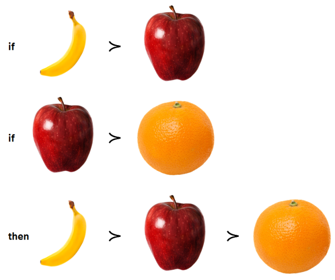
Weak stochastic transitivity demands that preferences be ordered and internally consistent. For example, if you prefer bananas over apples, and apples over oranges, then you must prefer bananas over oranges under the same conditions. Violating weak stochastic transitivity – e.g., choosing the orange instead of the banana – is irrational because you should always pick the option that maximizes utility. (The curved greater than symbol is best read as “is preferred to” in the diagram below.)

 

 

Strong stochastic transitivity
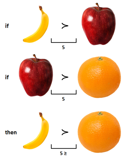
Strong stochastic transitivity requires consistency in the strength of the preference ordering. For example, if I prefer bananas over apples, and apples over oranges, the strength of my preferences for bananas over oranges (i.e., the weak transitive relationship) should be equal to or greater than the strength of my preference for bananas over apples, or apples over oranges. (In the diagram below, 5 represents the strength of preference.)

 

 

Independence of irrelevant alternatives
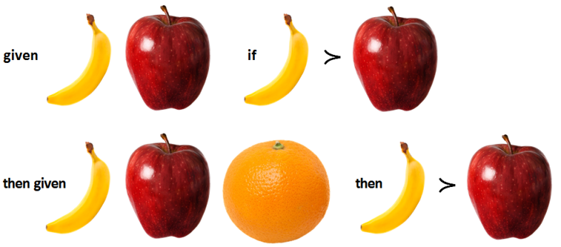
The independence of irrelevant alternatives axiom holds that a preference ordering must not change when the choice set is enlarged. For example, imagine that your are given the choice between a banana and an apple. Assume you prefer the banana. Now, imagine that I add an extra option, an orange. Regardless of how you feel about oranges, you can’t suddenly prefer apples over bananas. Adding an orange to the original banana and apple choice set is irrelevant to your preferences between bananas and apples. Whether you prefer apples or bananas is strictly a consideration between those two options, so your preferences between those options must be independent from other options, such as the orange.

 

 

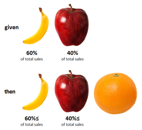
Regularity
Regularity, sometimes referred to as property α, is a stronger form of the independence of irrelevant alternatives. It’s best to think about regularity at the market level. Regularity holds that the absolute preference for an option cannot increase when options are added to the choice set. For example, imagine a market only comprised of bananas and apples, and assume that 60% of sales are for bananas and 40% are for apples. Now imagine we add oranges to this market. Regularity holds that the absolute number of bananas sold should not increase beyond the original 60% of absolute (total) sales in the pre-orange market. With the addition of oranges, the market share of apples and bananas should either maintain or decline, but never increase.

 

 

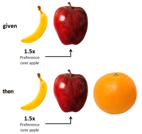
Constant-Ratio Rule
The constant-ratio rule is a weaker form of the independence of irrelevant alternatives. It demands that the ratio of preferences between choices (i.e., relative preferences) hold constant as the choice set expands. For example, in a market with bananas and apples where bananas are preferred at a 1.5x ratio to apples, the addition of oranges should not change the initial relative preference ratio of bananas over apples.

Defining rationality is challenging, but Nobel Prize-winning economist Herbert Simon has provided us with three ways to think about this important topic.

 

Substantive rationality concerns the degree to which a decision maximizes utility — or, from an evolutionary biology perspective, the degree to which it maximizes reproductive fitness. Evaluating substantive rationality requires a comparison between the content of a decision and the desired outcome. When economists speak of rationality, they’re usually referring to substantive rationality.

 

While substantive rationality is simple in concept, it’s nearly impossible to measure in practice. For example, we can’t quite answer the question that substantive rationality demands: “Given all the choices you could have made, was eating a banana the best one?” Still, substantive rationality is the logical theoretical yardstick for evaluating decisions.

 

In contrast, procedural rationality concerns the degree to which a decision is the outcome of a reasonable computational process. Procedural rationality requires consistency and coherence of preferences and choices. For example, a choice that is procedurally rational should abide by transitivity: if I prefer bananas to apples, and apples to oranges, then I should prefer bananas to oranges.  

 

Economists generally ignore procedural rationality and assume that we’ll abide by procedural axioms, such as transitivity. However, decades of research tells us that we break the fundamental rules that underlie procedural rationality: we resort to heuristics, fall prey to biases, and exhibit inconsistent preferences. As a result, psychologists are acutely interested in procedural rationality as a benchmark against which we can measure our systematic decision biases. 

 

It’s important to realize that our inability to abide by procedural rationality isn’t the only roadblock to substantive rationality. Even if we could achieve procedural rationality, the option space is often so vast that we cannot make an optimal decision — i.e., it is computationally intractable. For example, there are about 10¹²⁰ possible combinations in a chess game, which is many times larger than the number of atoms in the universe. With this understanding, we arrive at Simon’s concept of bounded rationality, which is defined as maximizing within the constraints of limited knowledge, limited time, and limited cognitive processing power.  

 

While no specific criteria exist to determine whether a decision is boundedly rational, it’s a helpful concept that frees us from the unattainable and unhelpful standards derived from neoclassical economics. Most importantly, it reminds us that when we discover departures from procedural rationality, we shouldn’t sound the alarm bells and decry the foibles of the mind. Sometimes we simply reach the limits of the universe.  

As I discussed in an earlier article that you should read for context, prospect theory has a wide range of implications on behavioral economics. One area in which prospect theory is particularly important is in the domain of mental accounting, which concerns how the way in which we think about and categorize financial activities can influence our choices.

 

Prospect theory tells us that value is reference-dependent. Thus, if we re-frame the reference point, we can modify the value of an event. Richard Thaler’s concept of “hedonic framing” in mental accounting [pdf] builds on this premise and offers four principles to maximize value:

 

 

1. Separate gains
What it means

Since the gain function is concave, we experience diminishing sensitivity to incremental increases. Ten gains of $100 feels better than one gain of $1,000. As a result, we can maximize the hedonic impact of gains by spreading them across separate temporal instances instead of aggregating them into a single event.

 

How to use it

• Give employees multiple smaller bonuses or raises over time (vs. one large bonus or raise)
• Order packages to arrive on different days; give gifts over time or wrapped in different wrapping paper
• Share good news over multiple conversations (vs. all at once)
• Split up pleasurable experiences (e.g., two 20 minute massages vs. one 40 minute massage; eat a bit of a bar of chocolate every day vs. all at once)

 

 

2. Combine losses
What it means

The loss function is convex, and as a result, we experience diminishing sensitivity to losses. A single loss of $10 feels less worse than 10 losses of $1. Thus, we can minimize the hedonic impact of losses by aggregating them into one episode.

 

How to use it

• Pay all of your bills on the same day each month
• Pay all taxes (federal, state, local) on one form and with one check
• Aggregate financial losses into one quarter; exit your low performing investments at once (there’s reasonable evidence that this occurs in practice [pdf])
• Share multiple instances of bad news at one time
• Group unpleasant activities into a single episode (e.g., go to the dentist and get your colonoscopy on the same day)

 

 

3. Combine smaller losses with larger gains
What it means

Since the value function is steeper for losses than for gains, we experience loss aversion. For example, we’re more upset losing $5 than happy gaining $5. The interaction of loss aversion with diminishing sensitivity for gains (i.e., diminishing marginal returns) means that we should integrate large gains with smaller losses to neutralize the disproportionate disutility from losses. For example, we feel better when we get a single gain of $95 than a gain of $100 paired with a loss of $5.

 

How to use it

• Charge small bank fees on the same day as large deposits
• Pay commuter fees out of your salary
• Communicate very good news at the same time as minor bad news (e.g., enhanced employee benefits paired with a 2% increase in the employee’s share of dental costs)

 

 

4. Separate smaller gains from larger losses
What it means

The value function for gains is concave and steepest near the origin. As a result, we should try to experience as many small gains as possible. We’ll miss out on the disproportionate impact of a small gain if we use it to slightly offset a large loss. Instead, we can maximize value by separating the small gain from the large loss. For example, we feel better with a small gain of $5 on one day with seemingly unrelated loss of $100 on the next day than a single integrated loss of $95.

 

How to use it

• Overpay your taxes and get a small refund; oversave for a vacation and return with some money left over
• Issue severance checks on a different day from when someone is fired
• Charge a higher price for a product and issue a rebate at a subsequent date

Prospect theory, outlined in 1979 by Kahneman & Tversky in what became one of the most cited papers in the social sciences [pdf], is the bedrock of modern behavioral economics. It’s often portrayed in the popular press as the instantiation of a phenomenon we can all intuit: the displeasure from losing $5 is worse than pleasure from gaining $5. This descriptive formulation belies the true power of the complex cognitive mechanics implied by prospect theory (e.g., the value function and the probability weighting function). Rather than describing the technical detail of these elements, we’ll instead focus on the three core features of risky choice derived from prospect theory, and talk about what they mean in plain English.

 

 

1. Value is relative to a reference point
What it means

Our perception of value is dependent on the relative change and not on the resulting (absolute) value.

 

Example

Person A starts out with $100K in assets and wins $900K in a lottery, and now has $1M to her name. Person B starts out with $2M and loses $1M, and now has $1M. Even though they have the same resulting net worth, person A will feel a lot better than person B.

 

Why it’s important

In Von Neumann-Morgenstern utility, which serves as the basis for expected utility theory (EUT), the end result of a gamble is the ultimate determinant of utility. Under EUT, whether the gamble is framed as a gain or a loss is irrelevant. In contrast, prospect theory holds that value is defined based on the relative change in wealth instead of the resulting levels of wealth.

 

 

2. Loss Aversion
What it means

The value function is steeper for losses than for gains.  As a result, we are much more sensitive to losses than gains of the same magnitude.

 

Example

If you lose $5, you’ll suffer a loss of utility that is greater than the gain in utility that you would feel from earning $5.

 

Why it’s important

Loss aversion causes risk aversion, which is when you prefer a gamble with a lower expected value at a higher probability to a gamble with a higher expected value at a lower probability. For example, most people prefer $20 with 100% certainty than a 50%/50% gamble of $50 or $0.

 

 

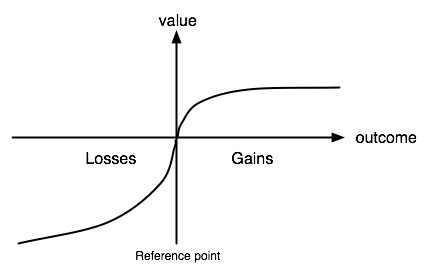
3. Diminishing Sensitivity for Losses and Gains
What it means

The value function is concave for gains, but convex for losses. As a result, the impact of an additional gain of $1 falls as the overall gain increases, and the impact of an additional loss of $1 falls as the overall loss increases. The degree of diminishment is equal for losses and gains.

 

Example

Replacing a $100 loss with a $110 loss has a greater impact than replacing a $1,000 loss with a $1,010 loss.  

 

Why it’s important

Diminishing sensitivity leads to risk aversion for gains (discussed above) and risk seeking for losses. For example, most people prefer a 50%/50% gamble between a loss of $0 and $1,000 than a certain loss of $500.